The purpose of this project was to create a framework for allowing robots to patrol an environment and engage in simple tasks with minimal human intervention. The 'Map Making' page shows a video of the hallway map being constructed and converted into a connected graph. The 'Person Following' page shows videos of a robot autonomously pursuing people that it is programmed to visually recognized. The 'Multi-robot Planning' page shows a video of robots autonomously responding to commands made through a custom GUI. The paper below shows some details about the obstacle avoidance, mapping, localization, and person following algorithms.
Behavior Set
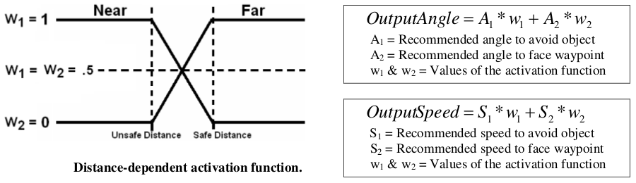
The robots in this project were coded with an obstacle avoidance behavior and a waypoint seeking behavior. A simple fuzzy system was used to fuse the output from these behaviors. Obstacle avoidance used laser range-finder information to identify objects that were within the path of the robot. The behavior output was a turn-angle away from the nearest object and a recommended speed that would allow safe completion of the maneuver . The waypoint seeking behavior (described below) used a graph-based map to produce a sequence of waypoints making a virtual path from the robot to its destination. The behavior output was a turn-angle toward the nearest waypoint and a speed that was always at maximum. The fuzzy system fused the two behaviors in a way that took the nearest obstacle into consideration. If the obstacle was dangerously close to the robot, the obstacle avoidance behavior was executed exclusively (Obstacle avoidance weight = 1, Waypoint seeking weight = 0). If the nearest obstacle was reasonably far from the robot, the waypoint seeking behavior was executed with full weight. If the object fell within the fuzzy region between near and far, the output angle and speed were a function of the fuzzy weight corresponding to the distance activation function shown below. This fuzzy system was used in all trials that involved waypoint seeking and person following.
Mapping & Navigation
The software used in this project was available as part of the "Simple Mapping Utilities (pmap)" from the Player software package (Howard, 2004). The pmap package provides several utilities for laser-based mapping in 2D
environments. The components are as follows:
1) Laser-stabilized odometry (lodo): Makes corrections to the robot's odometry readings so that current laser readings are most consistent with previously obtained readings.
2) Particle-filter-based-mapping (pmap): Uses a particle filter to maintain a set of possible robot trajectories and local maps that produce the best correspondence between the robot's laser readings and the global map.
3) Relaxation over local constraints (rmap): A post-processing step that uses an "iterated closed point algorithm” to refine a map using repeated observations of the same features. Provides a solution to the "loop closing" problem by looking for correspondences that occur when a robot returns to a location that it has already mapped.
4) Occupancy grid mapping (omap): Converts laser readings into an occupancy grid.
Though effective in simulated environments and in small real-world environments, the Player mapping software performed poorly in the hallway environment used in this project. Two major problems were encountered. First, odometry errors caused the long straight corridors to be mapped as curves. Second, the environment was too large, and the odometry errors were too great, for the rmap algorithm to complete the closure of the main loop.
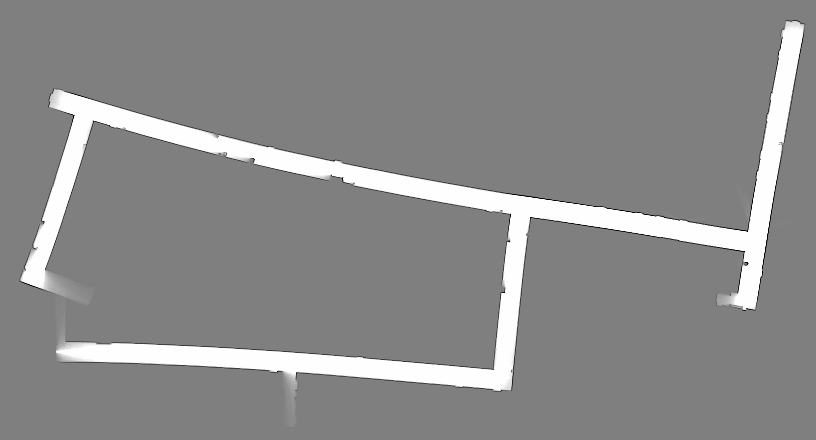
The results of the original Player software using a particle filter containing 200 particles.
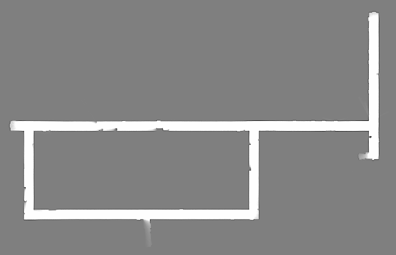
In response to these problems, an algorithm was developed that improved mapping speed and accuracy by making the reasonable assumption that walls are straight and lie either parallel or perpendicular to one another. If a building does not meet this criteria, the mapping system will resort to the original mapping algorithm. This assumption was applied as a secondary component of the particle filter. During map generation, a line-detection algorithm determines the linearity of incoming data. When linear regions are located, they are used to judge subsequent measurements. Measurements that are collinear or perpendicular with established lines are assigned higher accuracy readings, increasing the probability that those maps are maintained by the particle filter.
The results of the modified Player software using a particle filter containing only 20 particles (one tenth the number of particles used in the previous map). This reduction in tracked particles allowed mapping to take place in real-time on a robot. It should be noted that if this algorithm is applied to regions containing no linear segments, it will default to the standard mapping algorithm, though performance will degrade since significantly fewer particles are used.
Connected Graph Construction
Robots used the Player-provided localization software to estimate their location and orientation on the map. Waypoints represent target locations that the robot will actively seek. Waypoints can either be assigned manually by the user using a GUI (demonstrated in the 'Multi-robot Planning' scenario), or they can be autonomously placed on the map by a robot to mark the location of an observed object. For example, if the system identifies a person of interest, then a waypoint is created to mark that person's location. As the person moves through the environment, the coordinates of the waypoint are automatically adjusted. If the person leaves the robot's field of view, then the waypoint will remain at the person's last know position until visual contact is resumed. Since the robot is programmed to drive toward the waypoint, then this iterative process of seeking and updating will effectively cause the robot to "chase" the person of interest (demonstrated in the 'Person Following' scenario).
Although the Player software did provide waypoint-seeking functionality, the algorithm did not support on-line updates to a waypoint's position. Therefore, a new system had to be developed. For optimization, player's wave-front planning algorithm, was replaced by a much faster graph-based planner. The traditional wave-front planner operated by assigning a distance-to-target measurement to every traversable pixel on the map. If a target was in motion, all pixels must be updated at every iteration of movement. This is not insignificant given the nearly 40,000 elements involved in the hallway environment map. For comparison, the developed graph-based system could represent the same floor plan using only 8 nodes. Although this representation is particularly well suited for hallway floor-plans, it should be noted that it can be used for any environment. In addition to reducing storage and processing demands, a graph also increases the flexibility of the system. If a robot is attempting to navigate to one of the nodes and encounters an obstruction, it is relatively simple to eliminate the connection from the graph, while searching the remaining graph for the next-shortest route.
The idea behind our graph construction algorithm was to identify a set of nodes that correspond to intersections, dead-ends, and corners. An initial set of nodes was identified after iteratively eroding pixels from the perimeter of the map to form an image 'skeleton'. Interest points were located by counting the number of (4-way connected) pixels adjacent to each skeleton pixels. Skeleton pixels joined by only one other pixel are labeled end-points, while skeleton pixels joined by three or four other pixels are considered intersection pixels. The skeleton representation of the hallway environment is shown in the image below, with interest points marked using black and red circles.
A skeletonized representation of the hallway environment. Skeleton is shown in blue. Endpoint nodes are shown using black circles and intersection nodes are shown using red circles.
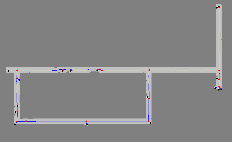
A connected graph is formed using skeleton pixels as a guide to identify associations between adjacent nodes. This graph is then simplified by using a distance threshold to remove nodes that contribute little to the shape of the graph. Nodes are eliminated if the distance between them and a wall, or the distance between them and another node are less than, or equal to, 1/4 the width of the hallway. As a final check of graph integrity, lines are drawn between every pair of connecting nodes (this represents 'line-of-sight'). If a line is found to leave the navigable portion of the map, additional 'corner' nodes are iteratively added until all connecting lines are contained by the map. If a non-intersection node can be removed without causing the adjacent nodes to violate the line-test, then that node is removed. The resulting simplified graph is shown in the image below.

A minimized connected-graph representation of the environment. Node connections are shown in blue. Endpoint nodes are shown using black circles and intersection and corner nodes are shown using red circles.
As a final step to making the connected-graph map, a fast-access array is made to associate every navigable pixel on the map to its nearest graph-node. A color representation of this array is shown below.
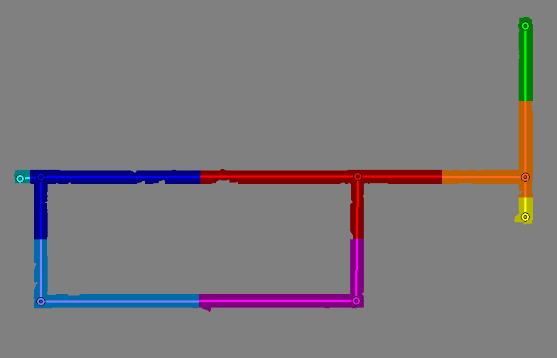
A reference array allows a robot to efficiently find the nearest graph node by using its location as a query. Graph nodes are represented by colored circles, with corresponding regions being illustrated using a similar color. Lines between nodes represent the graph connections.
Dynamic Waypoint Seeking
The algorithm for pursuing the waypoint is relatively simple when using the connected graph. The robot uses the Map-to-Graph Translation Array to identify the graph-node that is closest to its position in the environment (This is referred to as the primary-node and is always considered to be within the robot’s line-of-sight). It then goes through that node's adjacency list and identifies the connected nodes that are also within the robot’s line-of-sight (referred to as connected-nodes). As was mentioned previously, nodes are generated using the constraint that each node is within the line-of-sight of their adjacent nodes. This is done to simplify the way that a robot determines if a connecting node is within its own line-of-sight. Basically, if the angle between the connected-node and the primary-node is similar to the angle between the connected-node and the robot (allowable error is within the width of the hallway), then the connected-node is determined to be in the line-of-sight of the robot. The robot then stores the list of all node-pairs where both nodes in the pair are within its line-of-sight (all node-pairs will contain the primary-node and one connecting-node).
Once the robot establishes its own position among the nodes, it repeats the test on the waypoint. If the waypoint returns one of the same node-pairs as the robot, then the waypoint is considered to be within the robot’s line-of-sight and the robot will approach the waypoint directly (even if there is some error in this assumption, it will be close enough that the robot’s obstacle avoidance routine will ensure that a safe path is followed). If the waypoint is not within the robot’s line-of-sight, it will conduct a recursive search of the graph to identify the sequence of nodes that produces the shortest distance to the destination. The robot will then be directed toward the first node in that sequence. Since the graph search can be done extremely quickly, it is conducted at every time step. It should be noted that our definition of visibility ensures that before any node in the sequence is actually reached; subsequent nodes will always become visible. This ensures that the robot will not attempt to position itself at the exact location of each intermediate waypoint before continuing on to the next, thus producing a natural and efficient path through the environment.